Manual Reference Pages - M_calcomp (3)
NAME
M_calcomp(3fm) - [M_calcomp::INTRO] emulate old Calcomp graphics library (LICENSE:PD)
CONTENTS
Synopsis
Table Of Contents
Introduction
Calcomp Basic Software
Calcomp General Functional Software
Calcomp Scientific Functional Software
Applications Routines
Calcomp Code Migration Supplement
Introduction
Calcomp Basic Software
Example
A Sample Plotting Program
Calcomp General Functional Software
Calcomp Scientific Functional Software
Application Routines
Calcomp Manpages
Calcomp Setup
Calcomp Supplement
Moving Existing Calcomp Code
Record Of Revisions
Example
License
SYNOPSIS
THE CALCOMP GRAPHICS LIBRARY USER GUIDE
This is an interface that closely emulates a very early de-facto graphics standard called the "CALCOMP-compatible library" and is generally used to interface to older utilities that support CALCOMP interfaces, or to quickly resurrect codes that have CALCOMP calls in them. It is not recommended for new large code development.
The CALCOMP library is a simple set of FORTRAN callable graphic routines that allows users to quickly construct plots. It was historically used principally to interface to purchased vendor software that often supplied a "CALCOMP library interface", and for quick development of codes that generated XY plots (that is right -- products often could not produce graphics without being hooked up to the customer custom plotting interfaces!).
Consult the supplement at the end of this guide for specific guidelines on how to convert existing user and vendor CALCOMP code.
Revision 1.0.0: 07/01/91
TABLE OF CONTENTS
The following sections are available ....
INTRODUCTION
CALCOMP BASIC SOFTWARE
Sample Plotting Program
PLOT - Move or draw to specified point, establish plot origin, update pen position and terminate plotting PLOTS - Initialization, specify output file unit number FACTOR - Adjusts the overall size of the plot WHERE - Returns current pen location NFRAME - Ends current frame and re-origins pen position SYMBOL - Plots annotation (text) and special symbols NUMBER - Plot decimal equivalent of a floating point number SCALE - Determine starting value and scale for an array to be plotted on a graph AXIS - Draws an annotated linear graph axis LINE - Scale and plot a set of X,Y values NEWPEN - Select new pen color WIDTH - Set line thickness
CALCOMP GENERAL FUNCTIONAL SOFTWARE
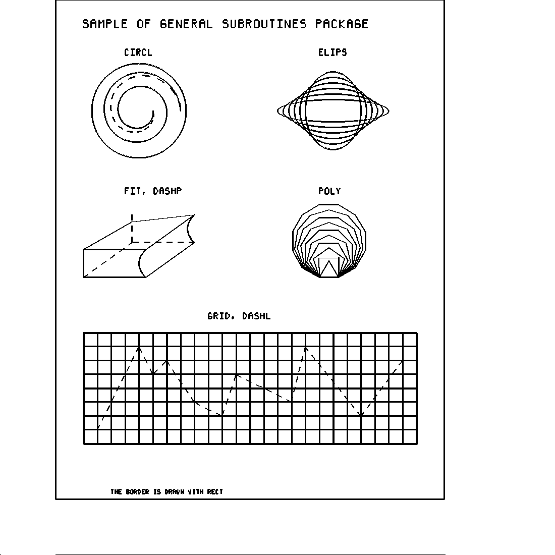
CIRCL - Draws a circle, arc, or spiral ELIPS - Draws an ellipse or elliptical (or circular) arc DASHL - Draws dashed line connecting a series of data points DASHP - Draws a dashed line to a specified point FIT - Draws a curve through three points GRID - Draws a linear grid POLY - Draws an equilateral polygon RECT - Draws a rectangle
CALCOMP SCIENTIFIC FUNCTIONAL SOFTWARE
CURVX - Draws a function of X over a given range CURVY - Draws a function of Y over a given range FLINE - Draws a smooth curve through a set of data points SMOOT - Draws a smooth curve through sequential data points SCALG - Performs scaling for logarithmic plotting LGAXS - Plots an annotated logarithmic axis LGLIN - Draws data in either log-log or semi-log mode POLAR - Draws data points using polar coordinates
APPLICATIONS ROUTINES
CNTOUR - Makes a contour plot
CALCOMP CODE MIGRATION SUPPLEMENT
INTRODUCTION
Other changes may be needed in existing CALCOMP code from vendors as CALCOMP has produced several versions of CALCOMP routines that vary in such ways as use of CHARACTER variables versus Hollerith, the number of parameters on SYMBOL calls, and the current pen position after a call to SYMBOL.This user guide describes the calling sequences and arguments for the FORTRAN-callable CALCOMP software subroutines. The routines do not produce a device dependent CALCOMP file but rather call the M_draw(3f) graphics module.
CALCOMP divides their routines into three categories:
Basic, General Function, and Scientific Function.Differences between the implemented routines and the standard CALCOMP routines are:
o All coordinate values should be greater than or equal to zero, and less than 100 inches. Values outside this range may result in unpredictable results (Negative values are possible if the frame coordinate origin is set first using the PLOT call).
o The metalanguage output filename is "pdf", and uses FORTRAN unit 50 unless an appropriate alternate value is specified in the PLOTS routine call. The output filename may be specified using the environment variable CALCOMP_PDF.
o A routine NFRAME is available for creating multiple frames for graphic devices other than pen plotters.
o Color is supported via the NEWPEN routine
o Line thickness is supported via the WIDTH routine
o Frames will not plot to true inches unless specific steps are taken in the generation and post-processing of the plot file.
The CALCOMP subroutines were written for use with CALCOMP pen plotters and originally worked in units of inches for the mapping of the plot directly to the output device. There are two classes of CALCOMP subroutines--those that accept user units and scale them to inches and those that require data to be directly in units of inches.
Table 1 lists the CALCOMP subroutines that fall into each class.
The main difference CALCOMP users will notice when using this CALCOMP library is that when the CALCOMP subroutines were incorporated into M_DRAW(3fm) the meaning of CALCOMP inches was altered to no longer mean a physical inch but just a unit-less measure (since M_DRAW(3fm) uses device-independent space and the graphics post processing procedures produce output for a number of graphics devices, some of which have a limited device space unlike pen plotters). THIS DIFFERENCE IS USUALLY ONLY OF SIGNIFICANCE TO USERS TRYING TO PRODUCE PLOTS USING TRUE INCHES.
The graphics post processing procedures use the CALCOMP inches to determine the aspect ratio of the plot, and the plot is made as large as possible for a given device while maintaining the aspect ratio specified by the user CALCOMP calls. A parameter called SIZE is included with most graphics post-processor procedures which facilitates the scaling of plots to a specific size in inches. An example program shows how to use these parameters to get consistent frames in as close as possible to true inches.
TABLE 1
Scaling versus Device units> Routines Which Routines Which Require > Perform Scaling Inches > of User Data to Inches (Data Must be Scaled to Inches) > ______________________ _______________________________ > > SCALE PLOT > AXIS WHERE > LINE SYMBOL > DASHL NUMBER > FLINE CIRCL > SCALG ELIPS > LGAXS DASHP > LGLIN FIT > POLAR GRID > POLY > RECT > CURVX > CURVY > SMOOT
CALCOMP BASIC SOFTWARE
The routines included in the CALCOMP Basic Software category are PLOT, PLOTS, FACTOR, WHERE, SYMBOL, NUMBER, SCALE, AXIS, LINE, WIDTH and NEWPEN. NFRAME, an enhancement, is included here because it performs a basic function.
Usually when examining existing CALCOMP code you will find it breaks down into two categories - that which produces XY plots and that which does almost everything in its own high-level routines and uses CALCOMP mostly just to draw lines with the PLOT command. Therefore you are likely not to need to be familiar with many of the CALCOMP routines described here.
The majority of graphic applications are intended to produce an XY-plot. Usually the production of these graphs requires only a combination of the routines PLOTS (initialize), SCALE, AXIS, LINE, NFRAME and PLOT (terminate). Additional text can be added with SYMBOL, and options such as frame borders and general line drawing might be added with PLOT calls.
When plotting requirements cannot be satisfied by using these subroutines, the code often calls the PLOT routine almost exclusively ( which basically draws a line or moves the pen directly in units of inches). This is often done by vendors so that it is very easy for them to interface to virtually any graphics library.
Two other routines are often found in programs that do not call the higher level routines (such as the axis and contour plot routines): follows:
FACTOR Adjusts the overall size of a plot. WHERE Returns the current pen location.
EXAMPLE
A SAMPLE PLOTTING PROGRAM
To illustrate the use of the CALCOMP routines, a sample program is provided which will produce the graph shown below. The only assumption made is that the 24 pairs of TIME and VOLTAGE data values are contained in a file of 24 records.
   program sample
   use M_calcomp
   !  Reserve space for 24 data values plus two additional locations
   !  required by the SCALE, AXIS, and LINE subroutines.
   dimension xarray(26),yarray(26)
   !  Perform initialization.
   call plots(0.0,10.0,0.0,10.0)
   !  Read 24 pairs of TIME and VOLTAGE from an input file into two arrays
   !  with names XARRAY and YARRAY.
   read (5,25)(xarray(i),yarray(i),i=1,24)
   25    format(2f6.2)
   !  Establish a new origin one-half inch higher than the point where the
   !  pen was initially placed so that the annotation of the TIME axis will
   !  fit between the axis and the edge of the plotting surface.
   call plot(0.0,0.5,-3)
   !  Compute scale factors for use in plotting the TIME values within a
   !  five-inch plotting area.
   call scale(xarray,5.0,24,1)
   !  Compute scale factors for use in plotting the VOLTAGE data values
   !  within a six-inch plotting area (i.e., the data pairs of TIME,
   !  VOLTAGE will plot within a five-by-six inch area).
   call scale(yarray,6.0,24,1)
   !  Draw the TIME axis (5 inches long), using the scale factors computed
   !  in statement 40 to determine the milliseconds at each inch along the
   !  TIME axis.
   call axis(0.0,0.0,’time in milliseconds’,-20,5.0,0.0,xarray(25),xarray(26))
   !  Draw the VOLTAGE axis (6 inches long) using the scale factors
   !  computed in statement 50 to determine the voltage at each inch along
   !  the VOLTAGE axis.
   call axis(0.0,0.0,’voltage’,7,6.0,90.0,yarray(25),yarray(26))
   !  Plot VOLTAGE vs TIME, drawing a line between each of the 24 scaled
   !  points and a symbol X at every other point.
   call line(xarray,yarray,24,1,2,4)
   !  Plot the first line of the graph title.
   call symbol(0.5,5.6,0.21,’performance test’,inteq,0.0,16)
   !  Plot the second line of the graph title.
   call symbol(0.5,5.2,0.14,’ref. no. 1623-46’,inteq,0.0,16)
   !  Terminate the plot.
   call nframe()
   !  Close the plot file.
   CALL PLOT(0.0,00.0,999)
   !  Terminate Program execution.
   end program sample
CALCOMP GENERAL FUNCTIONAL SOFTWARE
The routines included in the CALCOMP General Functional software category are CIRCL, DASHL, DASHP, ELIPS, FIT, GRID, POLY and RECT. These routines call the Basic routines and should be viewed as an extension of the Basic library rather than as a separate entity.
CALCOMP SCIENTIFIC FUNCTIONAL SOFTWARE
The routines included in the CALCOMP Scientific Functional software category are CURVX, CURVY, FLINE, LGAXS, LGLIN, POLAR, SCALG, and SMOOT. These routines call the Basic routines and should be viewed as an extension of the Basic library.
APPLICATION ROUTINES
The routines included in this category draw, on a single call, complete plots of types useful to engineers. They are not part of the software from CALCOMP, but they do use the Basic CALCOMP subroutines.
CNTOUR
CALCOMP MANPAGES
If the manpages have been installed properly, you should be able to list all the CALCOMP-related pages by entering
man -s 3m_calcomp -k .There should be a directory in the source for the GPF (General Purpose Fortran) collection that contains a collection of example CALCOMP programs in
PROGRAMS/CALCOMPYou can list all the manpages sorted by section using
   #!/bin/bash
   export MANWIDTH=80
   for NAME in $(man -s 3m_calcomp -k . |sort -k 4|awk ’{print $1}’)
   do
      man -s 3m_calcomp $NAME |col -b
   done
CALCOMP SETUP
Since this version of a CALCOMP-compatible library uses the M_draw(3f) graphic primitives, the same environment variables can be used to select the type and size of output. For example:
# where the M_draw(3f) font files are located export M_DRAW_FONTLIB=/usr/share/hershey# X11 # set output to Poskanzer pixel map format at specified size export M_DRAW_DEVICE=’x11’ # run a program demo_general
# There are many output formats available (Adobe PDF, PostScript, SVG, ...)
# POSKANZER ASCII FILES (one of the harder ones to use in this case) # set output to Poskanzer pixel map format at specified size export M_DRAW_DEVICE=’p3 850 1100’ # the name of the output file export M_DRAW_OUTPUT=calcomp.p3
# optionally set up the virtual size in inches of the calcomp drawing surface export CALCOMP_XMIN CALCOMP_XMAX CALCOMP_YMIN CALCOMP_YMAX CALCOMP_XMIN=0 CALCOMP_XMAX=8.5 CALCOMP_YMIN=0 CALCOMP_YMAX=11
# run a program demo_general # split pixmap file into individual drawings csplit -f P3. -k calcomp.p3 ’%^P3%’ ’/^P3/’ ’{999}’ 2>&1 >/dev/null
CALCOMP SUPPLEMENT
MOVING EXISTING CALCOMP CODE
The CALCOMP plot library emulates the interface originally leased from California Computer Products, Inc; and had been available in a very similar form on the old CDC 7600 Super Computers. Of course, this similarity is intentional. This library is trying to provide a consistent programming environment wherever possible.
All of the subroutines from the 7600 version of the CALCOMP library have been included in this version; although plots generated will not always look exactly the same as those produced on the 7600s.
The CALCOMP library is interfaced to locally developed routines (called primitives) which produce plots using the M_DRAW(3fm) module. This allows CALCOMP-based code to generate output which can be sent to any supported M_DRAW(3fm) output device.
CALCOMP is not the recommended graphics package for major new program development.
CALCOMP is being provided to meet certain special requirements:
1. To facilitate the migration of user code that already uses a CALCOMP-like package to new machines. 2. To support interfaces to non-inhouse code. Such code may often already support a set of CALCOMP-like calls. 3. Applications where a simple portable interface is more important than powerful graphics capabilities. There are no plans to provide local enhancements to CALCOMP, and capabilities such as high-level charting routines will not be made available with CALCOMP. Those involved in program conversions and development are urged to consider long-term graphics requirements in deciding which package to use (CALCOMP or an alternative).
The CALCOMP software was initially developed to drive only CALCOMP plotters. In general, the calls produced plots directly in inches (A call to draw a line one unit long produced a one-inch line on the plotter).
With the interfacing of CALCOMP to the M_DRAW(3f) module graphics system (which provides the ability to obtain output on a wide range of devices), the meaning of units in the CALCOMP library has undergone a change. CALCOMP Inches, therefore, may not translate directly into physical inches on a pen plotter.
Important differences exist between this CALCOMP and "standard" CALCOMP interfaces third-party software often provides interfaces to. The format of the following primary example program can be used as a guide as to how to nullify the affects of these differences.
DIFFERENCES FROM 7600 CALCOMP LIBRARIES1. For subroutines SYMBOL, AXIS, and LGAXS, the parameter used to specify text or title information (IBCD) has been changed to be type CHARACTER to be consistent with ANSI 77 FORTRAN. Data for these arguments should be changed to be type CHARACTER (although use of a Hollerith string or INTEGER array may currently work, their use is not recommended, and there are no plans to support this usage).
2. For subroutine SYMBOL on the 7600s, there is a "STANDARD" call (used to plot a text string) and a "SPECIAL" call (used to plot a single symbol). To Accommodate CHARACTER data and both versions of the call to SYMBOL, the calling sequence was modified to have 7 arguments. All programs being converted from the 7600 -MUST- make this change to the call to SYMBOL.
The new calling sequence is
CALL SYMBOL(XPAGE,YPAGE,HEIGHT,IBCD,INTEQ,ANGLE,NCHAR)
Where XPAGE, YPAGE, HEIGHT, and ANGLE are defined as on the 7600s, and the user guide can be consulted for details of their use.The last parameter NCHAR is used as a flag to specify whether a text string or a single symbol is being plotted. If NCHAR is less that zero, a single symbol is plotted regardless of the contents of IBCD. If NCHAR is equal to or greater than zero the string in IBCD is used (FAILURE TO SPECIFY THE PROPER VALUE FOR NCHAR, INTEQ OR IBCD WILL CAUSE ERRONEOUS RESULTS).
To use SYMBOL to plot text for titles, captions, or legends--
IBCD--Contains the text string as CHARACTER data.For example, the following call to SYMBOL will result in the charactersINTEQ--Should be set to 999 . (THE ACTUAL VALUE IS NOT USED FOR ANYTHING.)
NCHAR--Is the number of characters in IBCD.
         CHARACTER GRLBL*8
         GRLBL = ’TITLE 10’
         CALL SYMBOL(1.0,1.0,0.14,GRLBL,999,0.0,8)
To use SYMBOL to plot a single symbol or character--
IBCD-- A dummy CHARACTER variable or string should be used THE ACTUAL VALUE IS NOT USED FOR ANYTHING.)For example, the following call to SYMBOL will result in special symbol number 5 being output with its center at XY coordinates of (1.0,1.0).INTEQ--Contains the INTEGER EQUIVALENT of the desired symbol. If INTEQ has a value of 0 (zero) through 14, a centered symbol (where XPAGE and YPAGE specify the center of the symbol) is produced. The symbol table is unchanged from that on the 7600s, so the table on page 2-10 of the 7600 CALCOMP guide is still applicable.
NCHAR--Determines whether the pen is up or down during the move to XPAGE and YPAGE. (IT MUST BE NEGATIVE.)
When NCHAR is--
-1, the pen is UP during the move. -2 or less, the pen is DOWN during the move.
CALL SYMBOL(1.0,1.0,0.14,DUMMY,5,0.0,-1)
3. Because of interfacing the CALCOMP routines to the device dependent M_DRAW(3fm)-based post-processing procedures, some limit for the maximum plot size had to be established. For the CALCOMP library, a plot frame is limited to a maximum size in either the X or Y direction of 100 "CALCOMP inches". (The actual frame size on a particular output medium is dependent on the method of post- processing and the device selected.) Each plot frame is usually initialized by a call to subroutine PLOT with the third argument (IPEN) equal to -2 or -3. For example,
CALL PLOT(0.5,1.0,-3)Says to move 0.5 inches in the X-direction and 1.0 inch in the Y-direction before establishing a new origin. When establishing a new origin, all offsets are included inside the frame boundary, and therefore, they are part of the plot frame size. If any X or Y coordinate value (Plus the appropriate offset) exceeds the 100 inch limit, results are unpredictable. In programs where X and Y coordinate values exceed the scaling limit, a call to the CALCOMP routine FACTOR may be used to scale down the plot size appropriately. Each plot frame is terminated by a call to subroutine NFRAME; no additional offset is added here.
Knowledge of the plot frame size in the X and Y directions will be needed to scale pen plots to actual inches when the device dependent post processing procedures are available. The following example is provided to assist in understanding how the frame size is determined.
      >   PROGRAM CALTEST
      >   USE M_calcomp
      >   CALL PLOTS()           ! perform initialization
      >   CALL BORDER(8.5,11.0)  ! establish a consistent frame size
      >!  Calls to generate first plot go here
      >!  where all calls stay inside area established by border
      >!    .
      >!    .
      >   CALL NFRAME()          ! terminate first plot
      >   CALL BORDER(8.5,11.0)  ! establish a consistent frame size
      >!  In next plot negative values up to (-1,-2) are needed
      >   CALL PLOT(1.0,2.0,-3) ! establish origin for second plot
      >!  To stay in the border no numbers greater than XBORDER-1 in X
      >!  or YBORDER-2 can be used
      >!  Calls to generate second plot go here
      >!    .
      >!    .
      >   CALL NFRAME()          ! terminate second plot
      >   CALL PLOT(0.0,0.0,999)! close the plot file
      >   END PROGRAM CALTEST
      >   SUBROUTINE BORDER(XBORDER,YBORDER)
      >!  Must be called with same values throughout entire program
      >!  or not all frames will plot to same scale.
      >!  Draw a box inside of which all frames can appear
      >   CALL PLOT(XBORDER,0.0,    2)
      >   CALL PLOT(XBORDER,YBORDER,2)
      >   CALL PLOT(0.0,    YBORDER,2)
      >   CALL PLOT(0.0,    0.0,    2)
      >   END SUBROUTINE BORDER
4. All coordinate values (XPAGE, YPAGE for example) should be greater than or equal to zero relative to the original frame origin. Negative values will be clipped or might cause post-processor errors. (Although this was not a requirement on the 7600s, it is necessary because metafiles must contain only positive values and it would be very inefficient to store each frame’s data and then translate all the values to positive numbers once the frame was finished and the largest negative numbers in the frame could be identified.
6. Subroutine PLOTS must still be the first CALCOMP subroutine called. It performs various initialization functions and should be called only one time per program execution. Although some of the values are not used, they are maintained for compatibility purposes. 7. Subroutine CNTOUR (Which was developed at the Westinghouse Research Laboratories) is available in the CALCOMP library. The plot produced by CNTOUR will look different from that produced on the 7600s since the legend is placed at the top of the plot. If more that 20 contours are used, the legend could overwrite the plot. A limit of 6.5 inches must be observed for the height parameter (HGT).
RECORD OF REVISIONS
06/24/85 Preliminary release was made for COS. 07/11/89 The routine NEWPEN may be used to select color. 07/01/91 The first release of the documentation on UNICOS.
EXAMPLE
Sample program:
program demo_M_calcomp use M_calcomp ! 07/30/69 real :: x(104), y(104) character(len=40) :: msg integer,parameter :: kin = 50 equivalence(x(1),xl),(y(1),yl) 9007 format(7(1X,F9.3),F7.1) call make_c_qa4() ! create datafile f = 1.0 ipn = 2 call plots(0.0,10.0,0.0,10.0) !----------------------------------------------------------------------- open(unit=kin,file=’qa4.dat’,action="read") NEXTREAD: do read(kin,9001) nrec, msg 9001 format(1X,I2,7X,A40) write(*,*)’NREC=’,nrec,’MSG=’,trim(msg) select case(adjustl(msg)) !----------------------------------------------------------------------- case(’DATA’) do i = 1,nrec read(kin,9007) x(1),y(1),x(2),y(2),x(3),y(3),x(4),y(4) do j = 1,4 if(x(j).eq.0)then if(y(j).eq.0)then ipn = 3 cycle endif endif call plot(x(j),y(j),ipn) ipn = 2 enddo enddo !----------------------------------------------------------------------- case(’CIRCL’) do i = 1,nrec read(kin,9007) xl,yl,tho,thf,ro,rf,di call circl(xl,yl,tho,thf,ro,rf,di) enddo !----------------------------------------------------------------------- case(’DASHL’) do i = 1,nrec read(kin,9009) x(1),y(1),npts,inc 9009 format(2(1X,F9.3),1X,I3,7X,I1) j1 = inc+1 j2 = inc*npts+1-inc do j = j1,j2,inc read(kin,9007) x(j),y(j) enddo j = j2+inc x(j) = 0. y(j) = 0. j = j+inc x(j) = 1. y(j) = 1. call dashl(x,y,npts,inc) enddo !----------------------------------------------------------------------- case(’DASHP’) do i = 1,nrec read(kin,9007) xl,yl,d call dashp(xl,yl,d) enddo !----------------------------------------------------------------------- case(’ELIPS’) do i = 1,nrec read(kin,9012) xl,yl,rma,rmi,a,th0,thf,ipen 9012 format(7(1X,F9.3),1X,I1) call elips(xl,yl,rma,rmi,a,tho,thf,ipen) enddo !----------------------------------------------------------------------- case(’FIT’) do i = 1,nrec read(kin,9007) x(1),y(1),x(2),y(2),x(3),y(3) call fit(x(1),y(1),x(2),y(2),x(3),y(3)) enddo !----------------------------------------------------------------------- case(’GRID’) do i = 1,nrec read(kin,9014) xl,yl,dx,dy,nx,ny 9014 format(4(1X,F9.3),2(1X,I2,7X)) call grid(xl,yl,dx,dy,nx,ny) enddo !----------------------------------------------------------------------- case(’POLY’) do i = 1,nrec read(kin,9007) xl,yl,sl,sn,a call poly(xl,yl,sl,sn,a) enddo !----------------------------------------------------------------------- case(’RECT’) do i = 1,nrec read(kin,9021) xl,yl,h,w,a,ipen 9021 format(5(1X,F9.3),1X,I2) call rect(xl,yl,h,w,a,ipen) enddo !----------------------------------------------------------------------- case(’SYMBOL’) do i = 1,nrec read(kin,9016) xl,yl,h,msg,inc 9016 format(3(1X,F9.3), A40,1X,I3) read(kin,9017) a,nc 9017 format(1X,F9.3,1X,I2) if(inc.lt.0)cycle NEXTREAD call symbol(xl,yl,h,msg,inc,a,nc) enddo !----------------------------------------------------------------------- case(’1100’) do i = 1,nrec read(kin,9007) xl,yl call plot(xl,yl,-3) enddo !----------------------------------------------------------------------- case(’FACTOR’) do i = 1,nrec read(kin,9007) f call factor(f) enddo !----------------------------------------------------------------------- case(’END’) call factor(1.) call plot(20.,0.,999) exit NEXTREAD !----------------------------------------------------------------------- case default write(*,*)’unknown keyword ’,trim(msg) !----------------------------------------------------------------------- end select !----------------------------------------------------------------------- enddo NEXTREAD close(unit=kin,status=’delete’) !----------------------------------------------------------------------- containssubroutine make_c_qa4() integer,parameter :: io=40 open(unit=io,file=’qa4.dat’,action="write") write(io,’(a)’)’ 1 RECT’ write(io,’(a)’)’ 1. 1. 9. 7. 0. 3’ write(io,’(a)’)’ 7 SYMBOL’ write(io,’(a)’)’ 1.5 9.5 .14 SAMPLE OF GENERAL SUBROUTINES PACKAGE 999’ write(io,’(a)’)’ 0. 37’ write(io,’(a)’)’ 2.25 9. .105 CIRCL 999’ write(io,’(a)’)’ 0. 6’ write(io,’(a)’)’ 5.75 9. .105 ELIPS 999’ write(io,’(a)’)’ 0. 5’ write(io,’(a)’)’ 2.25 6.5 .105 FIT, DASHP 999’ write(io,’(a)’)’ 0. 11’ write(io,’(a)’)’ 5.75 6.5 .105 POLY 999’ write(io,’(a)’)’ 0. 4’ write(io,’(a)’)’ 3.75 4.25 .105 GRID, DASHL 999’ write(io,’(a)’)’ 0. 12’ write(io,’(a)’)’ 2. 1.1 .07 THE BORDER IS DRAWN WITH RECT 999’ write(io,’(a)’)’ 0. 29’ write(io,’(a)’)’ 3 CIRCL’ write(io,’(a)’)’ 3.25 8. 0. 720. .75 .25 0.’ write(io,’(a)’)’ 3.25 8. 0. 360. .75 .25 1.’ write(io,’(a)’)’ 3.35 8. 0. 360. .85 .85 0.’ write(io,’(a)’)’ 6 ELIPS’ write(io,’(a)’)’ 6.5 8. .5 .7 0. 0. 360. 3’ write(io,’(a)’)’ 6.6 8. .6 .6 0. 0. 360. 3’ write(io,’(a)’)’ 6.7 8. .7 .5 0. 0. 360. 3’ write(io,’(a)’)’ 6.8 8. .8 .4 0. 0. 360. 3’ write(io,’(a)’)’ 6.9 8. .9 .3 0. 0. 360. 3’ write(io,’(a)’)’ 7. 8. 1. .2 0. 0. 360. 3’ write(io,’(a)’)’ 3 DATA’ write(io,’(a)’)’ 0. 0. 1.5 5. 1.5 5.5 2.375 6.’ write(io,’(a)’)’ 3.5 6.125 2.625 5.5 1.5 5.5 0. 0.’ write(io,’(a)’)’ 1.5 5. 2.625 5. 3.5 5.625 0. 0.’ write(io,’(a)’)’ 1 DASHP’ write(io,’(a)’)’ 2.375 5.625 .1’ write(io,’(a)’)’ 1 DATA’ write(io,’(a)’)’ 1.5 5. 1.5 5. 1.5 5. 0. 0’ write(io,’(a)’)’ 2 DASHP’ write(io,’(a)’)’ 2.375 5.625 .1’ write(io,’(a)’)’ 2.375 6.125 .1’ write(io,’(a)’)’ 2 FIT’ write(io,’(a)’)’ 2.625 5. 2.5 5.25 2.625 5.5’ write(io,’(a)’)’ 3.5 5.625 3.375 5.875 3.5 6.125’ write(io,’(a)’)’ 10 POLY’ write(io,’(a)’)’ 5.75 5. .35 3. 0.’ write(io,’(a)’)’ 5.75 5. .35 4. 0.’ write(io,’(a)’)’ 5.75 5. .35 5. 0.’ write(io,’(a)’)’ 5.75 5. .35 6. 0.’ write(io,’(a)’)’ 5.75 5. .35 7. 0.’ write(io,’(a)’)’ 5.75 5. .35 8. 0.’ write(io,’(a)’)’ 5.75 5. .35 9. 0.’ write(io,’(a)’)’ 5.75 5. .35 10. 0.’ write(io,’(a)’)’ 5.75 5. .35 11. 0.’ write(io,’(a)’)’ 5.75 5. .35 12. 0.’ write(io,’(a)’)’ 2 GRID’ write(io,’(a)’)’ 1.5 2. .25 .25 24 8’ write(io,’(a)’)’ 1.51 1.99 1.5 1. 4 2’ write(io,’(a)’)’ 1 DASHL’ write(io,’(a)’)’ 1.75 2.25 11 1’ write(io,’(a)’)’ 2.5 3.75’ write(io,’(a)’)’ 2.75 3.25’ write(io,’(a)’)’ 3. 3.5’ write(io,’(a)’)’ 3.5 2.75’ write(io,’(a)’)’ 4. 2.5’ write(io,’(a)’)’ 4.25 3.25’ write(io,’(a)’)’ 5.25 2.75’ write(io,’(a)’)’ 5.5 3.75’ write(io,’(a)’)’ 6.5 2.5’ write(io,’(a)’)’ 7.25 3.5’ write(io,’(a)’)’ END’ close(unit=io) end subroutine make_c_qa4
end program demo_M_calcomp
LICENSE
Public Domain
| M_calcomp (3) | March 11, 2021 |